

캐글에서 미니 프로젝트를 가져왔다.
https://www.kaggle.com/datasets/sharmastic/gender-by-name
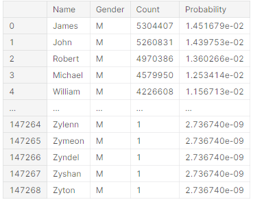
Gender By Name
Dataset for classification of Gender using name and corresponding attributes
www.kaggle.com
이름을 가지고 성별을 맞추는 문제였다.
처음에는 생각보다 쉽다고 여겼지만, 만만치 않았다.
사람을 이름을 컴퓨터가 인식할 수 있도록, 인코딩 하는 것 자체가 쉽지 않았다.
우리가 베이스라인으로 삼은 코드는 a에서 b까지 원핫인코딩 한 다음에, 중복된 이름을 제외하고 알파벳 하나하나에 인코딩 값을 부여하였다.
우리가 베이스라인으로 삼은 코드를 바탕으로, 다시 코딩 하려고 하였지만, 생각보다 쉽지 않았다.
우선 이것은 알고리즘 백그라운드가 완성되지 않아서, 생각대로 자유자재로 만들어지지가 않았다.
그리고 5명이 하는 조별 활동에서, 2명이 빠진 상태에서 3명이 하루만에 하는 프로젝트라 전략적 변경을 할 수 밖에 없었다.
그래서 우리는, 베이스라인을 바탕으로, 코드 하나하나 토론을 통해 이해를 하고, 여기 코드에서는 RNN만 모델로 돌렸지만, 더 나아가 비슷한 모델인 LSTM을 돌려보기로 하였다.
그리고 하이퍼파라미터나 모델 층을 개선하여, 정확도가 얼마나 개선되었는지 시각화하려는 것을 목표로 삼았다.
RNN 모델
def RNN_model(memory_size, vocab_size):
    model_RNN = tf.keras.Sequential([
        tf.keras.Input((None, vocab_size), ragged=True),
        tf.keras.layers.SimpleRNN(memory_size),
        tf.keras.layers.Dense(1, activation='sigmoid')
    ])
    model_RNN.summary()

    return model_RNN

# size of the "memory" of the RNN (size of the state vector passed to next time step)
MEMORY_SIZE = 50

RNN_model = RNN_model(MEMORY_SIZE, vocab.VOCAB_SIZE)
optimizer = tf.keras.optimizers.Adam(learning_rate=0.005)
RNN_model.compile(optimizer=optimizer, loss='binary_crossentropy', metrics=['acc'])
import time
start = time.time()
BATCH_SIZE = 4
NUM_EPOCHS = 30
# VALIDATION_SPLIT = 0.2
history_RNN = RNN_model.fit(x=training_data.inputs, y=training_data.targets, batch_size=BATCH_SIZE, epochs=NUM_EPOCHS)
print("time :", time.time() - start)import time 모듈을 사용하여 모델 학습 시간을 재어보았다.
RNN 모델 시각화
def plot_history(history):
    for key, values in history.items():
        plt.plot(values)
        plt.title(key)
        plt.xlabel('epoch')
        plt.show()

plot_history(history_RNN.history)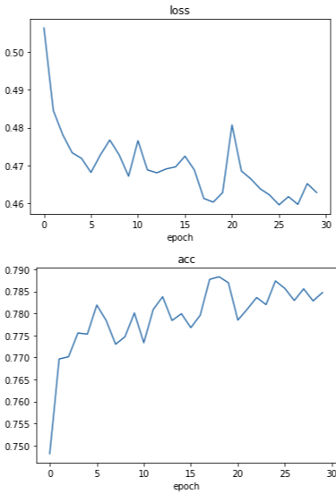
파라미터 시각화
1.먼저 RNN으로 파라미터를 시각화 해보았다.
%matplotlib inline
import numpy as np
import pandas as pd
import matplotlib.pyplot as plt
import plotly.express as px

df = pd.read_csv("RNN_Parameter.csv")
df

plt.figure(figsize=(8, 5))
df_learning_rate = df.loc[:4]
plt.plot(df_learning_rate['Learning rate'], df_learning_rate['Accuracy'], color='green')
plt.xlabel('Learning rate')
plt.ylabel('Accuracy')

plt.show()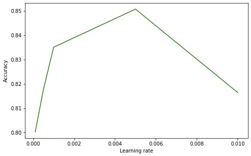
러닝레이트는 학습률로 무조건 높다고 혹은, 낮다고 좋은 것이 아니라 적정 크기에 최적의 정확도가 나타났다.
(러닝레이트를 제외하고 나머지 부분은 모두 고정시키고 구하였다.)
plt.figure(figsize=(8, 5))
df_batch_size=df[['Batch size','accuracy','Time']]
plt.plot(df_batch_size['Batch size'], df_batch_size['accuracy'], color='green')
plt.xlabel('Batch size')
plt.ylabel('Accuracy')

plt.show()
plt.figure(figsize=(8, 5))
plt.plot(df_batch_size['Batch size'], df_batch_size['Time'], color='green')
plt.xlabel('Batch size')
plt.ylabel('Time(s)')

plt.show()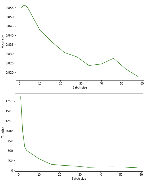
텍스트 관련 데이터이기 때문에, 배치사이즈가 낮을 수록 정확성의 향상을 기대할 수 있었다. 텍스트 데이터는 데이터 자체가 이미지 데이터에 비해서 가볍기 때문이다. 하지만 그에 반해 배치사이즈가 낮게 잡을수록 학습 시간은 더 오래걸렸다.
RNN으로 최종 학습한 정확도는 -> 0.7847이 나왔다.
LSTM 모델

LSTM 모델은 RNN모델의 개선한 모델로 Sequence가 지나갈수록 중요한 정보가 희석되는 문제를 cell을 만들어 중요한 기억을 기억하고 불필요한 기억을 없애는 형식으로 만들어졌다.
LSTM도 RNN과 같은 Sequence to sequence 모델이므로, RNN과 비슷하게 계층을 꾸며보았다.
def get_model(memory_size, vocab_size):
    model = tf.keras.Sequential([
        tf.keras.Input((None, vocab_size), ragged=True),
        tf.keras.layers.LSTM(memory_size),
        tf.keras.layers.Dense(1, activation='sigmoid')
    ])
    model.summary()

    return model

# size of the "memory" of the RNN (size of the state vector passed to next time step)
MEMORY_SIZE = 50

model = get_model(MEMORY_SIZE, vocab.VOCAB_SIZE)
optimizer = tf.keras.optimizers.Adam(learning_rate=0.005)

model.compile(optimizer=optimizer, loss='binary_crossentropy', metrics=['acc'])
BATCH_SIZE = 4
NUM_EPOCHS = 30
# VALIDATION_SPLIT = 0.2

history = model.fit(x=training_data.inputs, y=training_data.targets, batch_size=BATCH_SIZE, epochs=NUM_EPOCHS)
LSTM 모델 시각화
def plot_history(history):
    for key, values in history.items():
        plt.plot(values)
        plt.title(key)
        plt.xlabel('epoch')
        plt.show()

plot_history(history.history)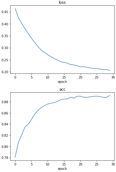
LSTM이 RNN보다 훨씬 더 깔끔하게 학습되는 것을 살펴볼 수 있다.
파라미터 시각화
1.LSTM 파라미터를 시각화 해보았습니다.
df = pd.read_csv("LSTM_parameter.csv")
df_learning_rate = df.loc[:4]
plt.figure(figsize=(8, 5))

plt.plot(df_learning_rate['Learning_rate'], df_learning_rate['accuracy_learning_rate'], color='green')
plt.xlabel('Learning rate')
plt.ylabel('Accuracy')

plt.show()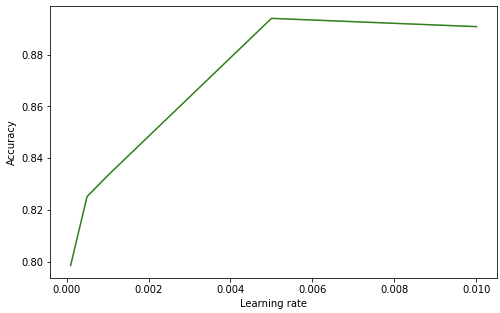
마찬가지로 적정 Learning rate에서 최적의 정확성을 보였다.
df_batch_size = df[['Batch_size','accuracy_batch_size']]
plt.plot(df_batch_size['Batch_size'], df_batch_size['accuracy_batch_size'], color='green')
plt.xlabel('Batch_size')
plt.ylabel('Accuracy')

plt.show()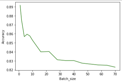
LSTM에서도 배치사이즈가 낮을수록 높은 정확성을 보였다.
def predict_gender(model, name):
    test_input = word2onehot(name.lower(), vocab)
    # add batch dimension of 1
    test_input = tf.reshape(test_input, (1, test_input.shape[0], test_input.shape[1]))

    return model.predict(test_input).flatten()[0]

name = 'Justin'
prob = predict_gender(model, name)

print(f"Model predicts that {name} is {float2gender(prob)} (output = {prob})")
prob = predict_gender(model, name)
Model predicts that Justin is M (output = 0.7318806052207947)
피드백 및 결론
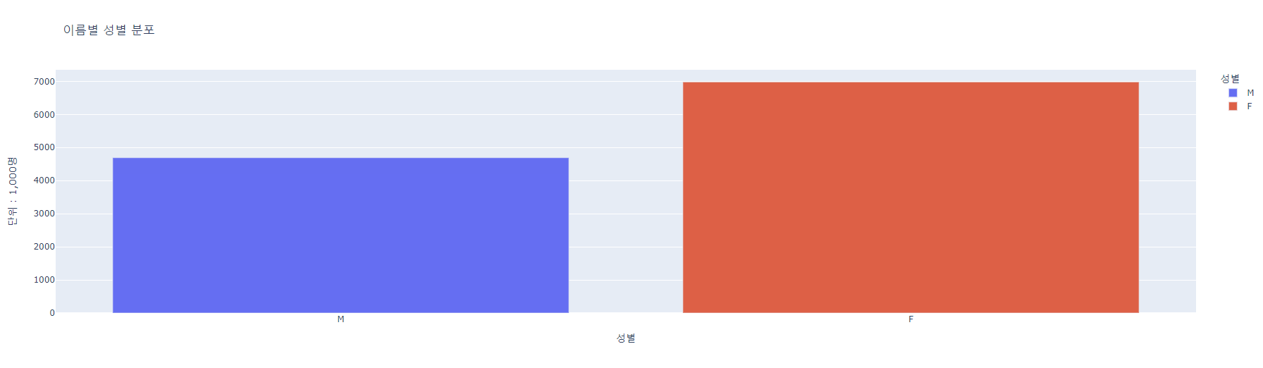
강사님께서 처음에 성별별 이름수를 시각화하는 대신에, 이름의 길이를 나타내는 시각화를 했으면 더 좋았을 것이라고 조언해 주셨다. 아무래도 이름의 길이가 길어질수록, LSTM의 효과가 더 커졌을 것이라고 말씀해 주셨다.
최종적으로 LSTM을 사용하여 캐글의 81%에서, 89.1%로 정확도를 향상시켰다.!
'플레이데이터 빅데이터 부트캠프 12기 > 머신러닝 & 딥러닝' 카테고리의 다른 글
| [플레이데이터 빅데이터 부트캠프]머신러닝 & 딥러닝 머신러닝 성능 평가 지표 정리 (0) | 2022.11.24 |
|---|---|
| [플레이데이터 빅데이터 부트캠프]머신러닝 & 딥러닝 텍스트 분석 기초 (0) | 2022.08.11 |
| [플레이데이터 빅데이터 부트캠프]머신러닝 & 딥러닝 RNN, LSTM (0) | 2022.08.11 |
| [플레이데이터 빅데이터 부트캠프]머신러닝 & 딥러닝 Teachable Machine (0) | 2022.08.10 |
| [플레이데이터 빅데이터 부트캠프]머신러닝 & 딥러닝 전이 학습 (0) | 2022.08.10 |